Example data — OpenMSK

← Back to OpenMSK

One real knee MRI, and every output OpenMSK produced from it. Use it to check that your own scans are the right kind of image before you upload anything, and to see what you get back.

⬇️ Example MRI NRRD image only ⬇️ MRI + all results Everything, zipped

Is my scan the right kind of image?

This is the question the example is really here to answer. OpenMSK's segmentation models were trained on gradient echo, fat-suppressed / water-excitation knee MRI — the bright-cartilage look you see in the example. If your images have roughly that contrast and cover the whole joint, they should work. If they look very different (a T1 spin echo, say, or a scan cropped to one compartment), expect the segmentation to be poor.

Three sagittal slices through the example knee, shown left to right from
the medial side to the lateral side. Each slice is displayed with the
front of the knee on the left and the top of the knee at the top. The
cartilage lining the femur and tibia is bright against dark bone marrow,
and the whole joint — femur, tibia, patella and the surrounding soft
tissue — is inside the field of view. — Three slices through the example scan: medial, central, lateral. This is the contrast to compare yours against — cartilage bright, bone marrow dark, and the whole joint in the field of view rather than cropped to one compartment.

The same three sagittal slices with the OpenMSK segmentation drawn on top
as a semi-transparent tint: bone in blue covering the femur, tibia and
patella; cartilage in orange as a thin curved band along each bone
surface; and meniscus in green as small wedges between the femur and
tibia in the medial and lateral slices. — The same three slices with the segmentation OpenMSK produced from them. Every structure it finds — bone, cartilage, meniscus — comes back as a label map, surface meshes, and thickness measurements.

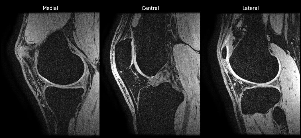
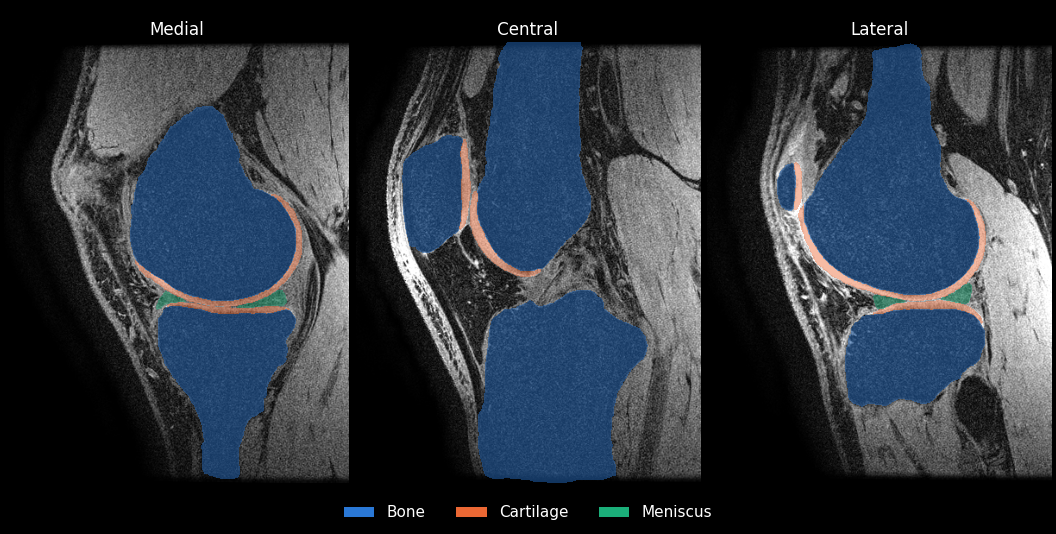
Download the image and open it next to one of your own in 3D Slicer, ITK-SNAP, or any NIfTI/NRRD viewer. Comparing them takes a minute and saves you a wasted upload.

Format	NRRD (`.nrrd`)
Contrast	Gradient echo, fat-sat / water excitation
Orientation	Sagittal
Dimensions	—
Voxel spacing	—
File size	—

You don't have to convert to NRRD

The example is NRRD because that is a compact single-file format, not because NRRD is required. All of these work:

NRRD — .nrrd
NIfTI — .nii or .nii.gz
DICOM — a whole series folder, zipped into a .zip. This is usually the easiest option, since it is what comes off the scanner or out of a PACS export. A single enhanced multi-frame .dcm file also works.

Uploads are capped at 150 MB. If a DICOM folder is larger than that, converting it to compressed NIfTI with dcm2niix usually gets well under the limit.

Upload DICOM if you want T2 maps. T2 relaxation mapping needs a qDESS acquisition, where T2 is computed from the ratio of two echoes together with gradient spoiling parameters stored in the DICOM headers. Converting to a single NRRD or NIfTI volume discards all of that, so T2 can only be computed from a qDESS DICOM series. Everything else — segmentation, meshes, thickness, shape model, BScore — works from any of the formats above.

What you get back

The bundle contains the image above plus every file the pipeline produced from it, so you can open the outputs before deciding whether to run your own data. In groups:

Segmentation Label maps in NIfTI and NRRD, as *_all-labels.* (femur, tibia, patella, their cartilages, and menisci) and *_subregions-labels.* (femoral cartilage split into anterior, weight-bearing, and posterior regions).

Surface meshes VTK surfaces per structure — femur_mesh.vtk, tibia_mesh.vtk, patella_mesh.vtk and the matching cartilage meshes. Cartilage thickness is stored on the bone meshes, not the cartilage ones: each bone surface carries a per-vertex thickness (mm) array (thickness is measured outward from the bone), plus a labels array giving the cartilage region each vertex belongs to. Colour femur_mesh.vtk by thickness (mm) in ParaView or 3D Slicer and you have a thickness map. The cartilage meshes are geometry only.

Cartilage thickness *_results.csv and *_results.json — mean, standard deviation, and median thickness in millimetres for each cartilage region.

Shape model and BScore Neural shape model fits, both bone-only and bone+cartilage. The reconstructed surfaces are the NSM_recon_* meshes; NSM_recon_params.json and NSM_bone_only_recon_params.json hold the latent vector, the fit error, and the BScore under the Bscore key.

Run settings job_manifest.json records the model and options used, so a run can be reproduced. _step_log.json lists which steps completed and which were skipped.

Reproducing this yourself

Download the image and upload it on the home page with the default options. You should get the same set of files. Small numeric differences between runs are normal — GPU floating-point arithmetic is not bit-for-bit reproducible — and results may also shift as the models and pipeline improve.

You can also skip the website entirely and run the same pipeline on your own machine. Install it from github.com/gattia/OpenMSK, in which case nothing leaves your computer.

Using this data

The scan is a maintainer's own knee, published deliberately. It carries no patient identifiers, and the files are named after this example rather than the original. You are welcome to use it for research and teaching, including in publications, provided you cite the paper below. It is not for clinical use — see the Terms of Use.

Goyal A, Belibi F, Sahani V, Pedersen R, Vainberg Y, Williams A, Chu C, Haddock B, Gold G, Chaudhari A, Kogan F, Gatti A. Automating Imaging Biomarker Analysis for Knee Osteoarthritis Using an Open-Source MRI-Based Deep Learning Pipeline. medRxiv 2025. doi:10.1101/2025.02.21.25322094

← Back to OpenMSK